Time Series forecasting with ARIMA part-2

Photo by Behnam Norouzi on Unsplash

Time series analysis is an important field in data science that deals with analyzing data points collected over time. In this blog, we will discuss time series analysis using Python, and demonstrate it with an example.

Time series data is often characterized by trends and patterns that can be analyzed and modeled to make predictions about future behavior. It is a widely used technique in various fields such as finance, economics, weather forecasting, and engineering.

To get started with time series analysis, we need to import a few libraries in Python, such as pandas, matplotlib, and statsmodels.

import pandas as pd
import matplotlib.pyplot as plt
from statsmodels.tsa.arima_model import ARIMA

# Load the dataset
data = pd.read_csv("AirPassengers.csv")

# Convert the date column to a datetime object
data['Month'] = pd.to_datetime(data['Month'])

# Set the date column as the index
data.set_index('Month', inplace=True)

# Plot the time series
plt.plot(data)
plt.xlabel('Year')
plt.ylabel('Passengers')
plt.show()

We will use the monthly airline passenger dataset for our example. This dataset contains the number of passengers who traveled by airplane each month from 1949 to 1960. We can load this dataset using the pandas library.

df = pd.read_csv('AirPassengers.csv', parse_dates=['Month'], index_col='Month')

The parse_dates argument is used to parse the dates from the CSV file, and the index_col argument is used to set the date as the index of the dataframe.

Next, we can visualize the data using a line chart.

plt.plot(df)
plt.xlabel('Year')
plt.ylabel('Passenger Count')
plt.show()

The resulting chart shows a clear increasing trend over time, with seasonality and periodicity.

To analyze the time series data, we need to decompose it into its trend, seasonal, and residual components. We can do this using the statsmodels library.

from statsmodels.tsa.seasonal import seasonal_decompose
decomposition = seasonal_decompose(df)
trend = decomposition.trend
seasonal = decomposition.seasonal
residual = decomposition.resid

The trend component represents the long-term increase or decrease in the data. The seasonal component represents the periodic fluctuations in the data. The residual component represents the random fluctuations in the data that cannot be explained by the trend or seasonal components.

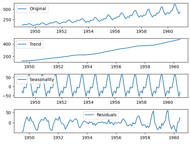
We can visualize the decomposed components using the following code.

plt.subplot(411)
plt.plot(df, label='Original')
plt.legend(loc='best')
plt.subplot(412)
plt.plot(trend, label='Trend')
plt.legend(loc='best')
plt.subplot(413)
plt.plot(seasonal,label='Seasonality')
plt.legend(loc='best')
plt.subplot(414)
plt.plot(residual, label='Residuals')
plt.legend(loc='best')
plt.tight_layout()
plt.show()

The resulting chart shows the original data and its decomposed components.

Now, we can use the ARIMA model to make predictions about the future behavior of the time series data. ARIMA stands for AutoRegressive Integrated Moving Average, and it is a commonly used model for time series analysis.

We can train an ARIMA model on our dataset using the following code.

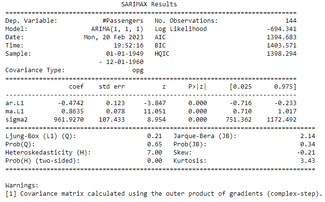
model = ARIMA(df, order=(1, 1, 1))
model_fit = model.fit(disp=0)
print(model_fit.summary())

The order argument is used to set the parameters of the ARIMA model. The first parameter is the order of the autoregressive (AR) component, the second parameter is the order of the integrated (I) component, and the third parameter is the order of the moving average (MA) component.

The model summary shows the coefficients of the model and the goodness of fit.

To make prediction of future dates or next 12 months use model.forecast function and pass steps(future periods)

# Make predictions for the next 12 months
forecast = model_fit.forecast(steps=12)

# Print the forecasted sales data
print(forecast)

Output

1961-01-01    475.735059
1961-02-01    454.996073
1961-03-01    464.830415
1961-04-01    460.167010
1961-05-01    462.378378
1961-06-01    461.329756
1961-07-01    461.827008
1961-08-01    461.591213
1961-09-01    461.703026
1961-10-01    461.650005
1961-11-01    461.675148
1961-12-01    461.663225
Freq: MS, Name: predicted_mean, dtype: float64

Here a github repo for this example:

https://github.com/chicks2014/Time-Series-Analysis-101

Conclusion

In this blog, we have explored the basics functions of time series analysis in Python. Time series analysis is an important tool for understanding trends, patterns, and behaviors in data that vary over time.

If you didn’t read my first part on time series analysis, I would suggest to read basic of time series first from here.

Time Series analysis and Forecasting for beginners part-1

If you like the article and would like to support me make sure to:

• 👏 Clap for the story (50 claps) and follow me 👉
• 📰 View more content on my medium profile
• 🔔 Follow Me: LinkedIn | Medium | GitHub | Twitter